Neural Networks with C# - part 2

Download Sample

A High Level Understanding of Backpropagation Learning

Backpropagation is a technique used to help a feedforward neural networks learn or improve the accuracy of it's output based on the expected output of the learning sample set. That is to say, we will have a set of sample inputs with their expected outputs and then use that set to make adjustments in for the weights of our neuron associations (again I like to call them axons). This approach effectively solves the problem of how to update hidden layers.

The Math Basics for Backpropagation Learning

http://www.youtube.com/watch?v=nz3NYD73H6E&p=3EA65335EAC29EE8

1. ri is the error for the nth node of the ith layer. Furthermore, r is only for the output layer; it is simply the difference between the expected output and the output (see Neuron.CalcDelta() in example download). vi is the values calculated during the normal feedforward algorithms (see part 1). Φ' will be explained in equation 4. δi is the calculated change for neuron n within the ith layer.
2. Critical: This is much like equation 1 with some very distinct differences. You may notice that instead of using r, the error is calculated by the sum of the jth delta with the weighted association axons of the nth neuron with the jth layer.
3. This equation is the gradient or calculated change of weights. Or in other words, this is where we make the learned changes. η is simply a learning rate between 0 and 1. y is the original input values calculated from the axon for the nth neuron during the feedforward calculation.
4. This is the inverse or derivative activation function for either sigmoid or hyperbolic tangent functions (depends on whichever activation function was used for the neurons).

As mentioned in part 1, n is referring to the nth node in a series of node calculations from input to output. Also, i and j simply note the distinction between one layer and another.

<< back to part 1

Download Sample

Neural Networks with C# - part 1

Download Sample

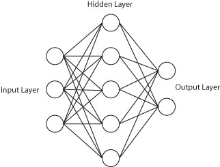
Neural networks and artificial intelligence is a fairly large topic. As such I will limit this article to a direct and simple example of creating a neural network with C#. Of course there are many other good examples, however I hope to provide simple code for those who are attempting to learn about neural networks. This example uses a standard hidden layer feedforward with backpropagation learning algorithm type of network.

A High Level Understanding

The type of neural network discussed in this article is one that has an input layer, one or more hidden layers, and an output layer. Below are two examples of potential neural networks.

Because of the obvious correlation between the cognitive thought process of the brain and an attempt to create a mathematical simulated model of it (thanks to John Von Neumann), like the term neural in neural networks, each node in the network is likewise called a neuron. The associate links between nodes I like to call axons (not officially called that, but I like it since it keeps with the whole biological brain naming conventions).

The Math Basics of a Feedforward Network

http://www.youtube.com/watch?v=nz3NYD73H6E&p=3EA65335EAC29EE8

1. vj is the input values for the jth layer. wji is the axon connectors 0 thru m from the ith layer to the jth layer.
2. y is the input values for the jth layer. This is calculated by passing the calculated value of node n coming from the ith layer to the activation function Φ(x).
3. Φ(x) is the activation function using either a sigmoid function or a hyperbolic tangent function (I prefer tanh because it better handles negative values).

It should further be noted that n is referring to the nth node in a series of node calculations from input to output. Also, i and j simply note the distinction between one layer and another.

I highly recommend watching Prof. S. Sengupta lectures for deriving these equations.

See part 2 >>

Download Sample